Page contents
How do I calculate the flow rate of a pipe under gravity flow?
When the outlet of a pipe is lower than the surface of the tank feeding it, the fluid flows by gravity and the flow rate settles by itself at the value for which the available head H is entirely consumed by the acceleration of the fluid and by the head losses: from Bernoulli, ρ g H = ½ ρ V² × (1 + Σζ + λ L / D), hence V = √(2 g H / (1 + Σζ + λ L/D)) and Q = V π D²/4. Since the friction factor λ itself depends on the velocity through the Reynolds number, you iterate: start from an estimated λ, calculate V, then the Reynolds number, then λ from Colebrook, and repeat until convergence, in two or three passes. Worked example below: drop 2 m, 80 mm pipe, 5 m long, roughness 1 mm, sharp-edged inlet (ζ = 0.5), water at 20 °C: λ = 0.041, V = 3.10 m/s, Q = 56 m³/h, i.e. 15.6 l/s. The box below links to the flow-velocity-diameter and major head loss calculators that let you carry out this iteration; Mecaflux Pro3D solves it automatically.
Gravity flow formulas
- H: drop between the free surface of the tank and the pipe outlet, in m; ρ g H is the available static pressure, in Pa (19,620 Pa for 2 m of water)
- ½ ρ V²: dynamic pressure at the outlet, in Pa, energy carried away by the jet; V: velocity in the pipe, in m/s; ρ: density, in kg/m³
- λ L/D: major head losses, λ from Colebrook according to the Reynolds number and roughness, L length and D bore in m
- Σζ: sum of the minor loss coefficients: sharp-edged inlet 0.5, rounded inlet 0.05, bend 0.2 to 0.3, open valve 0.1 to 0.3; the outlet is already accounted for by the dynamic pressure
- Q: flow rate, in m³/s (× 3,600 for m³/h, × 1,000 for l/s)
Iterations of the example: H = 2 m, D = 80 mm, L = 5 m, ε = 1 mm, inlet ζ = 0.5, water at 20 °C
| Pass | Assumed λ | Velocity V | Reynolds Re | Recalculated λ | Flow rate Q |
|---|---|---|---|---|---|
| 1 | 0.020 (estimate) | 3.78 m/s | 301,000 | 0.0411 | 68.4 m³/h |
| 2 | 0.0411 | 3.10 m/s | 247,600 | 0.0411 | 56.2 m³/h |
| 3 | 0.0411 | 3.10 m/s | 247,500 | 0.0411 | 56.2 m³/h (converged) |
| Balance | static pressure 19,585 Pa | = dynamic 4,810 Pa | + inlet 2,405 Pa | + friction 12,370 Pa | 15.6 l/s |
Gravity flow rate against drop and diameter (L = 5 m, ε = 1 mm, ζ = 0.5)
| Drop H (D = 80 mm) | Flow rate Q | Diameter D (H = 2 m) | Flow rate Q |
|---|---|---|---|
| 0.5 m | 28.0 m³/h | 50 mm | 17.5 m³/h |
| 1 m | 39.7 m³/h | 80 mm | 56.2 m³/h |
| 2 m | 56.2 m³/h | 100 mm | 96.0 m³/h |
| 5 m | 88.9 m³/h | 150 mm | 247 m³/h |
| 10 m | 125.7 m³/h |
Detailed explanations and calculation in Mecaflux
- Calculate the flow in a pipe with a vertical drop (gravity flow):
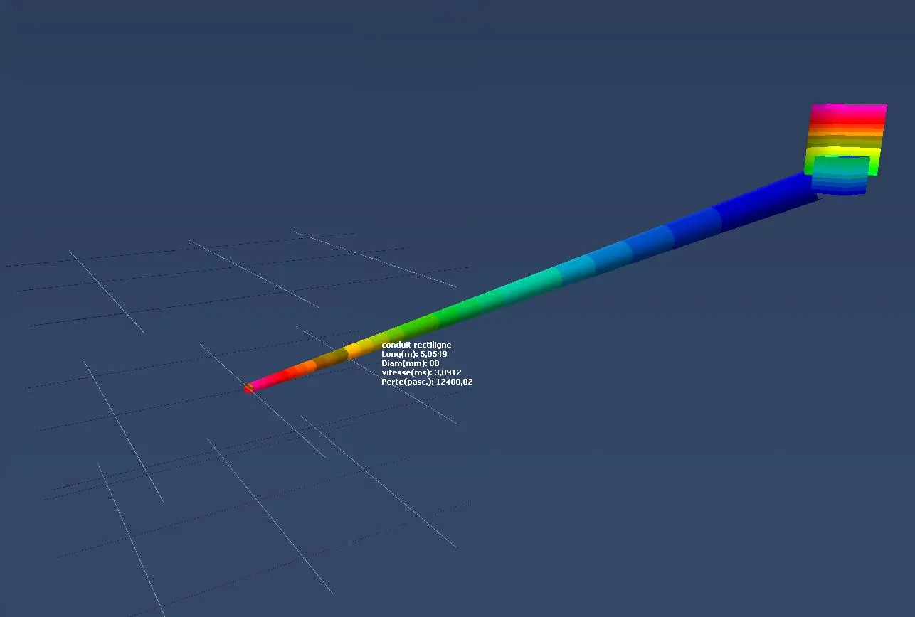
Here we explain the method of calculation of flow in a pipe with a slope (pressure losses are calculated with software or tables)
If the entry point of the network is higher than the outlet point, gravity flow is possible. This type of water intake generates a flow, depending on the three forms of energy pressure:
- the height of elevation (static pressure)
- the pressure losses (head loss energy lost)
- fluid velocity (dynamic pressure)
The flow in the conduit is reached, When the energy pressures are balanced between the entry point (A) and output (B) of the fluid (see Bernoulli):
- Energy inlet = P.stat A + P.dyn A
- Energy outlet = P.stat B+ P.dyn B
- Energy lost = Minor and Major head loss
with :
P.stat A= Static pressure at the entry point (pascals)
P.dyn A= Dynamic pressure at the entry point (pascals)
P.stat B= Static pressure at the outlet (pascals)
P.dyn B= Dynamic pressure at the outlet (pascals)
Pressure losses= Minor and Major head loss (pascals)
Energy in = energy out + energy lost
- Example of calculation of flow duct :
The flow will be one that balances the equation:
P.stat A + p.dyn A = P.stat B + p.dyn B + head loss
Reminder:
dynamic pressure (pascal) = 0,5 x ρ x V²
Static pressure (pascal) = ρ x 9,81 x H
With :
ρ= Fluid density in Kg/M³ (for water will be taken ρ=1000 KG/m³)
V=fluid velocity m/sec = flow M³/h * section m²
H altitude with the zero point inlet (from the surface of the water intake)
At the input, the hydrostatic pressure is zero (Altitude = 0) and the dynamic pressure is zero (fluid velocity collected in a lake for example = 0)therefore :
P.stat B + p.dyn B + head loss= 0
P.stat B= ρ x 9,81 x H = 1000 x 9,81 x (-2)= -19 620 pascals
it gives:
p.dynB + head loss= 19 620 pascals
The flow rate will be that which generates the pressure losses and a dynamic pressure being equal to the static pressure -19 620 pascals
p.dyn B = 0,5 x ρ x V² = 0,5 x 1000 x 9,81 x V²
head loss = Minor and Major head loss to the desired flow (we use tables or software to determine the major head loss in 5 meters pipe of roughness 1mm, and minor head loss will be neglected if we do not have software)
Some ittérations, calculations of losses, and dynamic pressures, taking the values of flow, allow us to determine the flow balancing equation: p.dynB + head loss= -19 620 pascals
Tutorial calculation flow network Mecaflux Pro 3D
The difficulty with this type of problem is :
- evaluation of head loss as it evolves according to the flow in a non-linear equation (see colebrook) which is solved with the Newton method or reading charts
- The necessity to repeatedly calculate to find the solution convergence, or draws a curve for pressure drop...
but here we will use a computer with mecaflux pro3D who perform these tasks in a few milliseconds:
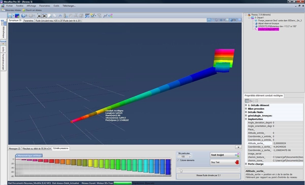
Frequently asked questions
Why is iteration needed to find the flow rate?
Because the unknown, the velocity, appears on both sides: the head losses depend on V² but also on the friction factor λ, which depends on the Reynolds number, hence on V. The equation has no direct solution; it is solved by successive approximations, which converge very quickly because λ varies little with the Reynolds number in rough turbulent flow (in the example λ is already exact at the second pass). You can also plot the head loss curve against flow rate with the calculator and read the flow rate at which it reaches the available head, or let a program such as Mecaflux Pro3D do the solving.
Should minor head losses be included?
Yes as soon as the pipe is short, because they then weigh as much as friction: in the example the sharp-edged inlet alone (ζ = 0.5) brings the flow rate from 60 to 56 m³/h, and a bend or a valve would take more off. The outlet, however, is not counted on top: the kinetic energy of the jet ½ ρ V² is already in the balance (it is the term 1 in the bracket). If the pipe discharges into a tank where the fluid comes to rest, that energy is lost in the same way and the result does not change.
How does the flow rate vary with drop, length and roughness?
The flow rate grows as the square root of the drop when losses dominate: going from 2 to 5 m of head only gains 58 %. It falls with the pipe length: 50 m instead of 5 m divide the flow rate of the example by 2.6. It grows strongly with the diameter, roughly as D2.5: a 100 mm pipe instead of 80 mm delivers 70 % more. Finally a smooth pipe (PVC, ε = 0.007 mm) delivers noticeably more than a rough or encrusted one: 32 against 22 m³/h over 50 m in the example.
How do I calculate the gravity flow rate of my own water intake or pipe?
Mecaflux Pro3D, as a stand-alone licence, solves this calculation automatically: you draw the pipe, its fittings and the drop in 3D, and the software iterates on the head losses to find the equilibrium flow rate, as the example on this page shows. Mecaflux Standard calculates the head losses of each section to carry out the iteration by hand. For a water intake, a turbine or a gravity network to design or check, Mecaflux carries out the study of your project and delivers the calculation report, or offers training on the software applied to your own installation.